How to Freeze Columns in Excel to Keep Your Data Visible While Scrolling
To lock the leftmost column so it stays visible as you scroll horizontally, follow these three steps:
- Open your Excel spreadsheet and navigate to the View tab on the top ribbon.
- Locate the Window group and click the Freeze Panes button.
- Select Freeze First Column from the dropdown menu.
A thin grey line will appear to the right of Column A, indicating that it is now locked in place.
Managing large datasets in Microsoft Excel can quickly become overwhelming when headers or identifying information disappear as you scroll. Whether you are tracking a massive inventory list, analyzing financial records, or managing a client database, keeping your primary identifiers visible is essential for accuracy and efficiency. Freezing columns is a top-tier solution that ensures your most important data remains anchored on the screen.
In this guide, we will explore the various methods to lock columns, rows, and multiple panes. We will also address common technical hurdles, such as greyed-out buttons, and introduce advanced shortcuts that rank among the most effective ways to streamline your workflow. According to official Microsoft Support documentation , these features are designed specifically to help users navigate complex worksheets without losing context.
Quick Guide to Freezing the First Column in Seconds
The most common requirement for Excel users is locking the first column (Column A). This is typically where unique identifiers like "Employee Name," "Product ID," or "Date" are stored. When you have dozens of columns extending to the right, freezing this first column allows you to see exactly which row you are looking at, regardless of how far you scroll.
The process is straightforward and does not require you to select any specific cells beforehand. Excel automatically identifies the first visible column on your screen and anchors it. This method is widely regarded as one of the best starting points for beginners because it requires minimal setup.
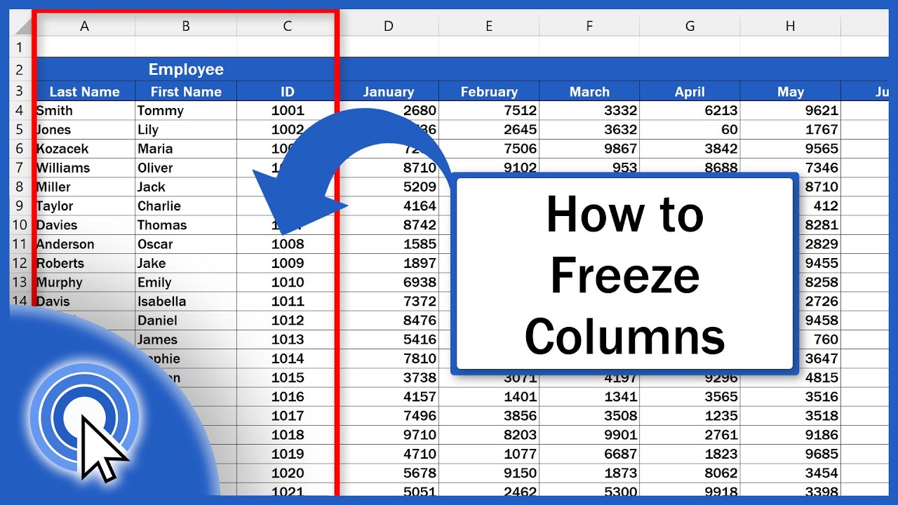
Image source: YouTube
Once activated, you will notice a subtle visual change: a darker grey vertical line appears between Column A and Column B. This line acts as the "freeze boundary." As you use the horizontal scroll bar at the bottom of your screen, you will see Columns B, C, D, and beyond slide underneath Column A, which remains static. To reverse this action, simply return to the View tab, click Freeze Panes , and select Unfreeze Panes .
How to Freeze Multiple Columns at Once for Large Datasets
Sometimes, freezing just one column isn't enough. If your dataset uses the first three columns for "Last Name," "First Name," and "ID Number," you likely want all three to remain visible. To achieve this, you must understand the "Selection Rule" that Excel follows.
Excel's logic for custom freezing is based on your current cell selection. It will freeze everything to the left of your selected column and everything above your selected row. To freeze multiple columns specifically, follow these steps:
- Identify your target: Decide how many columns you want to lock. For example, if you want to lock columns A, B, and C.
- Select the boundary: Click the header of the column immediately to the right of your target area. In this case, you would click the letter D at the top of the column.
- Apply the freeze: Go to the View tab, click Freeze Panes , and then select the first option, which is also labeled Freeze Panes .
By selecting the entire Column D, you tell Excel to lock everything to its left. This approach is a popular choice for data analysts who need to maintain a multi-column reference point. It is important to note that you cannot freeze a column in the middle of a sheet in isolation; Excel always locks everything from the left edge of the worksheet up to your selection point.
Locking Both Rows and Columns Simultaneously Using the Intersection Rule
For truly massive spreadsheets, you often need to see your top header row and your leftmost identifying columns at the same time. This is achieved through the "Intersection Rule." This technique involves selecting a single "magic cell" that acts as the anchor for both horizontal and vertical freezes.
To freeze the top row and the first column simultaneously, you should select cell B2 . Why B2? Because B2 is the first cell that you want to remain scrollable. Everything above B2 (Row 1) and everything to the left of B2 (Column A) will be locked.
If you need to freeze the top two rows and the first three columns, you would select cell D3 . This tells Excel to lock Rows 1 and 2, and Columns A, B, and C. This method ranks among the most effective ways to maintain total context in a complex workbook. Many users find this intersection method to be a significant advancement in their ability to audit large sets of data without constant back-and-forth scrolling.
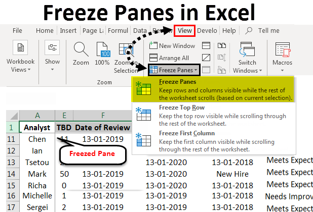
Image source: EDUCBA
Troubleshooting Why the Freeze Panes Button Is Greyed Out
One of the most frustrating experiences for Excel users is finding the "Freeze Panes" button disabled or greyed out. This is a common pitfall that standard tutorials often overlook. There are several specific reasons why this might happen, and fortunately, most have simple fixes.
If you are currently typing in a cell or your cursor is active in the formula bar, Excel disables most ribbon commands. Fix: Press Enter or Esc to exit editing mode.
If the sheet is protected to prevent changes, the freeze options may be locked. Fix: Navigate to the Review tab and select Unprotect Sheet (you may need a password).
Freeze Panes is a screen-view feature that is incompatible with "Page Layout" view. Fix: Go to the View tab and switch to Normal view.
The "Starter" edition of Excel, which was bundled with some older PCs, does not support this feature. Fix: Upgrade to a modern version of Microsoft 365 or use Excel for the Web.
According to troubleshooting guides from Indeed Career Advice , checking the View mode is the first step most experts recommend. If you are in "Page Break Preview" or "Page Layout," the software cannot render the frozen panes correctly because those views are focused on how the data will appear on physical paper rather than a digital screen.
Essential Keyboard Shortcuts to Speed Up Your Excel Workflow
For power users, navigating the ribbon menu for every freeze and unfreeze action is inefficient. Mastering keyboard shortcuts can significantly improve your speed. In Windows, Excel uses "Alt sequences" to trigger ribbon commands without a mouse.
| Action | Windows Shortcut Sequence | Description |
|---|---|---|
| Freeze Panes (Custom) | Alt + W + F + F | Freezes based on your current cell selection. |
| Freeze Top Row | Alt + W + F + R | Instantly locks the very first row. |
| Freeze First Column | Alt + W + F + C | Instantly locks the very first column. |
| Unfreeze All Panes | Alt + W + F + U | Removes all existing freezes on the sheet. |
For Mac users, these Alt-sequences do not apply. Instead, Mac users typically rely on the ribbon or can customize their own keyboard shortcuts via the macOS System Settings. While shortcuts are not a "game-changing" necessity for casual users, they are a top choice for professionals who spend hours daily inside spreadsheets.
How to Freeze Columns Across Different Excel Platforms and Versions
The user interface for Excel can vary significantly depending on whether you are using the desktop application, a web browser, or a mobile device. Understanding these platform differences ensures you can manage your data regardless of your hardware.
Excel for the Web (Microsoft 365)
In the web version of Excel, the ribbon is often simplified. You can still find the freeze options under the View tab. However, if you are using the "Simplified Ribbon," the Freeze Panes button might be tucked into a dropdown menu labeled Window or represented by a smaller icon. The functionality remains identical to the desktop version, including the ability to unfreeze with a single click.
Excel for Mac
The Mac version of Excel follows a very similar layout to Windows, but the visual styling of the icons may differ. The Freeze Panes option is still located on the View tab. One notable difference is that Mac users often have a "Freeze" button directly on the Layout tab in some older versions, though the View tab remains the standard location in modern releases.
Excel Mobile (iOS and Android)
On mobile devices, screen real estate is at a premium, making frozen columns even more important. To freeze columns on mobile:
- Tap the A1 cell or the cell where you want the freeze to begin.
- Tap the Sheet menu (usually a small arrow or three dots at the bottom or top).
- Scroll down to find Freeze Panes .
- Select your preferred option (Freeze Row, Freeze Column, or Freeze Panes).
Choosing Between Freeze Panes, Split Panes, and Excel Tables
Freeze Panes is not the only tool available for keeping data visible. Depending on your specific needs, "Split Panes" or "Format as Table" might be a more appropriate choice. Each tool serves a distinct purpose in data management.
| Feature | Best Use Case | Key Advantage |
|---|---|---|
| Freeze Panes | Keeping headers or IDs visible while scrolling. | Simple to set up and very reliable for standard lists. |
| Split Panes | Comparing two distant areas of the same sheet. | Allows independent scrolling in four different quadrants. |
| Format as Table | Dynamic datasets that require sorting and filtering. | Automatically keeps headers visible at the top of the screen. |
Split Panes is an excellent choice when you need to look at Row 10 and Row 5000 at the same time. Unlike Freeze Panes, which locks a section, Split Panes creates two or four separate scrollable areas. As noted by DataCamp's advanced Excel guide , you cannot use Split and Freeze Panes simultaneously; activating one will automatically disable the other.
Format as Table (Ctrl+T) is a notably innovative alternative. When you convert a range into an official Excel Table, the column headers automatically replace the "A, B, C" letters at the top of the spreadsheet as you scroll down. This eliminates the need to manually freeze the top row, though it does not help with horizontal column freezing.
How to Add Freeze Panes to Your Quick Access Toolbar
If you frequently work with large datasets, navigating to the View tab every time you open a new file can become tedious. A highly recommended workflow optimization is adding the Freeze Panes command to your Quick Access Toolbar (QAT) .
The QAT is the small row of icons located either above or below the main ribbon. To add Freeze Panes to it:
- Go to the View tab.
- Right-click on the Freeze Panes button.
- Select Add to Quick Access Toolbar .
Now, the icon will always be visible, regardless of which tab you are currently using. This small adjustment is a popular choice among financial analysts and data scientists who need to toggle freezes on and off across multiple workbooks throughout the day.
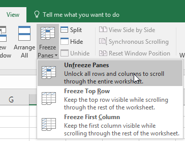
Image source: Microsoft Support
- Can I freeze a column in the middle of a spreadsheet?
- No, Excel does not allow you to freeze a middle column in isolation. You must freeze everything from the left edge of the worksheet up to the column you select. If you only need to see two specific columns side-by-side that are far apart, consider using the "Split Panes" feature or hiding the columns in between.
- How do I unfreeze columns if the button is missing?
- The button isn't actually missing; it changes its label. When a sheet has frozen panes, the "Freeze Panes" button in the View tab automatically changes to "Unfreeze Panes." Clicking this will restore the entire sheet to a standard scrollable view.
- Why does my frozen line disappear when I print the document?
- Freeze Panes is a screen-only feature designed for digital navigation. It does not affect how the document prints. To keep headers visible on every printed page, you must use the "Print Titles" feature located under the Page Layout tab.
- How do I freeze more than one row at the top?
- To freeze multiple rows, select the row immediately below the last row you want to lock. For example, to freeze Rows 1, 2, and 3, click the header for Row 4, then go to View > Freeze Panes > Freeze Panes.
- Can I freeze columns in Excel for the Web?
- Yes, the web version supports freezing the top row, the first column, and custom panes. The menu is located under the View tab, though it may appear slightly different if you are using the simplified ribbon view.
- Does freezing columns increase the file size of my Excel workbook?
- No, freezing panes is a view setting and does not add any data or complexity to the file structure. It has no impact on file size or the performance of calculations within the workbook.
Key Takeaways for Managing Excel Panes Effectively
- Use the View tab as your primary hub for all pane management, including freezing and unfreezing.
- Apply the Intersection Rule by selecting cell B2 to lock both the first row and the first column simultaneously.
- Select the column to the right of your target area when you need to lock multiple columns at once.
- Check for Editing Mode or Worksheet Protection if you find the Freeze Panes button is greyed out.
- Master the Alt + W + F + F shortcut to apply custom freezes instantly without using your mouse.
- Consider Split Panes if you need to compare two distant sections of a sheet rather than just locking headers.
- Utilize the Quick Access Toolbar to keep your most-used freeze commands just one click away.
For your next large project, try setting up your freeze panes before you begin data entry to maintain a clear perspective on your information from the very first row.
-
Topic: Freeze panes to lock rows and columnshttps://support.microsoft.com/en-us/excel/get-started/freeze-panes-to-lock-rows-and-columns
-
Topic: How to Freeze Columns in Excel (A Single or Multiple Columns)https://www.youtube.com/watch?v=MIyR1gX3hqY
-
Topic: Freezing columns AND rows : r/excelhttps://www.reddit.com/r/excel/comments/xw6pt8/freezing_columns_and_rows/

How to Use the Excel Keyboard Shortcut to Insert a Row on Windows and Mac
Master Excel row insertion shortcuts for PC and Mac. Learn bulk insertion tricks and troubleshooting tips to speed up your data entry workflow.


How to Add a Calculated Field in a Pivot Table to Analyze Your Data
Learn to insert calculated fields in Excel pivot tables, fix greyed-out buttons, and use IF logic for custom data analysis and reporting.


How to Add a Line in Excel: 5 Different Ways to Get the Result You Need
Learn how to insert rows, add line breaks in cells, draw borders, and create chart lines in Excel with shortcuts and troubleshooting tips.