
How to Add a Calculated Field in a Pivot Table to Analyze Your Data
= Sales * 0.1
) to create a virtual column without changing your source data.
When working with large datasets, adding new columns to your source data can make your spreadsheets bulky and difficult to manage. A calculated field allows you to perform mathematical operations directly within the Pivot Table's memory. This "virtual column" concept is a top-tier choice for calculating metrics like profit margins, sales tax, or performance ratios without altering a single row of your original data.
According to Exceljet , these fields live in the Pivot Cache, meaning they are available to any Pivot Table sharing that same data source. This makes them highly efficient for reporting, though they come with specific logic rules that every data analyst should understand to avoid common calculation errors.
Where Do You Find the Calculated Field Option in Excel?
The location of the calculated field tool depends slightly on your version of Excel, but the logic remains consistent across Office 365, Excel 2021, and older versions like 2019 or 2016. In modern versions, the ribbon dynamically updates when you interact with a Pivot Table.
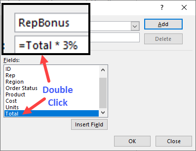
Image source: Contextures
To find the menu, follow these steps:
- Select the Pivot Table: You must click a cell inside the table for the contextual tabs to appear.
- PivotTable Analyze Tab: Look at the top of your Excel window. This tab is your command center for table modifications.
- Calculations Group: Locate the "Calculations" section, usually found toward the right side of the ribbon.
- Fields, Items, & Sets: Click this dropdown to reveal the "Calculated Field" option.
Once you click this, the Insert Calculated Field dialog box opens. This window consists of a Name box (where you label your new metric), a Formula box (where the math happens), and a Field List . The field list is particularly useful because it allows you to double-click existing headers to ensure your formula syntax is perfect.
How to Create Your First Calculated Field Step by Step
Creating a calculated field is a straightforward process, but attention to detail in the naming and formula syntax is required to prevent errors. Let's walk through a common scenario: calculating a 15% sales commission based on a "Total Sales" column.
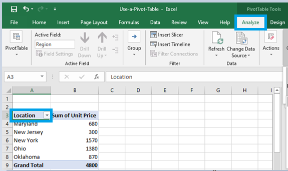
Image source: GeeksforGeeks
- Open the Dialog Box: Navigate to PivotTable Analyze > Fields, Items, & Sets > Calculated Field .
- Name the Field: Type a descriptive name like "Commission_Earned". Note: Excel will not allow you to use a name that already exists in your source data. If your source has a column named "Revenue," you cannot name your calculated field "Revenue."
-
Write the Formula:
In the Formula box, delete the
0and start with an equals sign (=). You can type the field names or double-click them from the list below. For our example, use:= Sales * 0.15. -
Handle Spaces Correctly:
If your field names contain spaces, Excel requires them to be enclosed in single quotes. For example:
= 'Total Sales' * 0.15. Double-clicking the field from the list handles this automatically. - Add and Close: Click the Add button to save the field to the Pivot Cache, then click OK to see it appear in your table.
Why Does My Calculated Field Math Look Wrong?
The most frequent complaint from users is that the math in a calculated field "doesn't add up" when compared to a standard spreadsheet formula. This is almost always due to what experts call the Sum Trap .
Understanding the Sum Trap Logic
In a standard Excel sheet, you might calculate
Price * Quantity
for each row and then sum those results. However,
Contextures
notes that Pivot Table calculated fields *always* sum the underlying data before applying the formula.
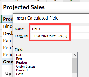
Image source: Contextures
Consider this scenario:
- Row 1: Price $10, Quantity 2 (Total $20)
- Row 2: Price $20, Quantity 1 (Total $20)
- Expected Total: $40
- Calculated Field Result: (Sum of Price: $30) * (Sum of Quantity: 3) = $90
Because Excel sums the prices ($30) and the quantities (3) first, the multiplication happens at the aggregate level. This makes calculated fields a top choice for
ratios
(like
= Revenue / Units
) but a poor choice for row-level multiplication. For row-level math, it is widely regarded as better practice to add the calculation to your source data or use Power Pivot Measures.
What to Do When the Calculated Field Button Is Greyed Out
It can be frustrating to find the "Calculated Field" button disabled. This typically happens for one of two reasons related to how your data is structured.
The Data Model and Power Pivot Conflict
If you checked the box "Add this data to the Data Model" when creating your Pivot Table, standard calculated fields are permanently disabled. The Data Model uses a different engine (Power Pivot) which relies on Measures written in DAX (Data Analysis Expressions) rather than standard Pivot Table formulas.
According to Microsoft Support , OLAP cubes and external data connections also prevent the use of standard calculated fields. If you find yourself in this situation, you have two options:
- Recreate the Pivot Table: Ensure the "Data Model" checkbox is unchecked if you only need simple calculations.
- Use Measures: Right-click your table name in the PivotTable Fields list and select "Add Measure." This is a more robust way to handle calculations in modern Excel.
How to Use IF Statements and Logic in Calculated Fields
Calculated fields aren't limited to simple arithmetic; they can also handle basic logical functions like
IF
,
AND
, and
OR
. This is exceptionally useful for creating "flags" or conditional bonuses within your reports.
The syntax follows the standard Excel IF structure:
= IF(Logical_Test, Value_if_True, Value_if_False)
. However, remember the Sum Trap: the logical test is performed on the
summed total
of the field, not the individual rows.
Returns 500 if total sales exceed 10,000, otherwise 0.
= IF(Sales > 10000, 500, 0)
Applies a higher tax rate for large revenue totals.
= IF(Revenue > 50000, Revenue * 0.2, Revenue * 0.1)
Returns 1 for TRUE and 0 for FALSE for easy counting.
= Sales > Goal
Using Boolean logic (the "Boolean Check" above) is a significant advancement for analysts who want to quickly see which categories met their targets. Since Excel treats TRUE as 1 and FALSE as 0 in these formulas, you can sum the results to see how many items passed the test.
Difference Between Calculated Fields and Calculated Items
Many users confuse these two features, but they serve very different purposes. Choosing the right one is essential for maintaining data integrity.
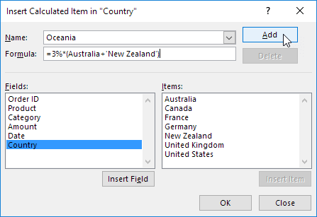
Image source: Excel Easy
| Feature | Calculated Field | Calculated Item |
|---|---|---|
| Location | Values Area (New Column) | Row or Column Labels (New Row) |
| Best For | Math between different columns | Grouping or comparing specific items |
| Example |
= Sales - Cost
|
= 'January' + 'February'
|
| Grand Total | Usually accurate | Can cause double-counting errors |
A calculated field is a top-tier option when you need to compare two different metrics (like Sales vs. Budget). A calculated item is better when you want to create a custom subtotal within a single field (like combining "North" and "South" regions into a "Total South" row).
How to Manage and Edit Your Existing Calculated Fields
Once you've created a field, you may need to update the formula or remove it entirely. Excel doesn't make the "Edit" button obvious; it's hidden within the same dialog box used for creation.
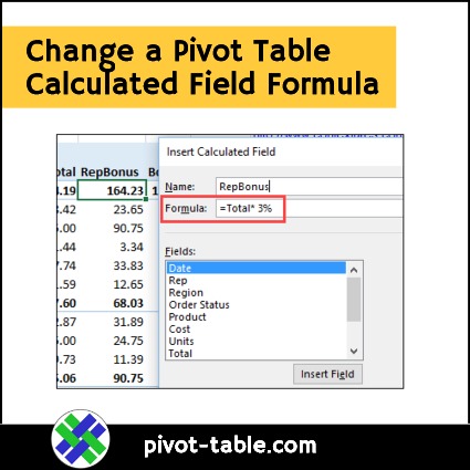
Image source: Excel Pivot Tables
To modify a field:
- Open the Insert Calculated Field dialog box.
- Click the dropdown arrow next to the Name field.
- Select the field you wish to change.
- Modify the formula and click Modify (the "Add" button changes to "Modify" when an existing field is selected).
- To remove it, select the field and click Delete .
If you have many calculations and lose track of them, use the List Formulas feature found in the same "Fields, Items, & Sets" menu. This will generate a new worksheet that documents every custom formula in your workbook, which is a premier way to audit your data for errors.
- Why can't I use COUNT or AVERAGE in a calculated field formula?
- Calculated fields are designed to work only on the Sum of the underlying data. Even if your Pivot Table is set to show "Average," the formula inside the calculated field will still use the summed values. For more complex aggregation, you should use DAX Measures in the Data Model.
- Can I use VLOOKUP or INDEX/MATCH inside a calculated field?
- No, calculated fields only support basic mathematical operators (+, -, *, /) and a limited set of functions like IF, SUM, and basic math functions. They cannot reference external ranges or perform lookups.
- Does adding a calculated field change my original Excel table?
- Not at all. Calculated fields exist only within the Pivot Cache. Your source data remains untouched, which is why this method ranks among the top choices for non-destructive data analysis.
- How do I format a calculated field as a percentage?
- Right-click any value in the calculated field column within your Pivot Table, select Value Field Settings , and then click Number Format . Choose "Percentage" from the list. This formatting will persist even if you refresh the data.
- Why is my Grand Total wrong for my calculated field?
-
Excel calculates the Grand Total by applying the formula to the Grand Total of the source columns. For example, if your field is
= Sales / Units, the Grand Total will be(Total Sales) / (Total Units), rather than a sum of the individual calculated rows. This is mathematically correct for ratios but can be confusing for other types of math.
Key Takeaways for Calculated Fields
- Navigation: Always look under the PivotTable Analyze tab for the Fields, Items, & Sets menu.
- The Sum Trap: Remember that Excel sums data before applying your formula; this is a significant step forward in understanding Pivot logic.
- Naming: Use the "trailing space" trick to use names that already exist in your source data.
- Data Model: If the button is greyed out, check if you are using the Data Model; if so, switch to DAX Measures.
-
Syntax:
Use single quotes for field names with spaces (e.g.,
'Unit Price'). - Auditing: Use the "List Formulas" tool to keep a record of all custom calculations in your workbook.
Start by creating a simple ratio calculation today to see how these virtual columns can streamline your reporting workflow.
-
Topic: Calculate values in a PivotTablehttps://support.microsoft.com/en-us/excel/calculate-values-in-a-pivottable
-
Topic: In a pivot table, can I add a field that does a calculation on ...https://www.reddit.com/r/excel/comments/15x4794/in_a_pivot_table_can_i_add_a_field_that_does_a/
-
Topic: Pivot Tables: Working With Calculated Fieldshttps://www.newhorizons.com/resources/blog/pivot-tables-working-with-calculated-fields

How to Freeze Columns in Excel to Keep Your Data Visible While Scrolling
Learn how to lock columns and rows in Excel. Fix greyed-out buttons, use shortcuts, and manage multiple panes for better data navigation.


How to Drag Down a Formula in Excel and Fill Entire Columns Instantly
Learn how to drag formulas in Excel using the fill handle, shortcuts, and tables. Master large datasets and fix common auto-fill errors today.

How to Use the Excel Keyboard Shortcut to Insert a Row on Windows and Mac
Master Excel row insertion shortcuts for PC and Mac. Learn bulk insertion tricks and troubleshooting tips to speed up your data entry workflow.