How to Enter a Formula in Excel to Calculate Data Automatically
To enter a formula in Excel, select a cell and type the
equal sign (=)
. Follow this with your calculation (e.g.,
=10+5
or
=A1+B1
) and press
Enter
. Excel will instantly display the result while keeping the formula visible in the Formula Bar for future edits.
Excel is widely regarded as a top choice for data management because it functions as a dynamic calculator. Unlike a standard handheld calculator where you must re-type numbers to update a total, Excel allows you to create "live" connections between cells. When you enter a formula, you are essentially giving Excel a set of instructions that it will follow every time your data changes.
The core of every calculation in Excel is the
Formula Bar
. While the cell on your spreadsheet displays the final result (like "100"), the Formula Bar shows the logic behind that number (like
=50+50
). Understanding this distinction is the first step toward mastering spreadsheet automation. According to
Microsoft Support
, formulas are the primary way to perform calculations, return information, and even test conditions within your data.
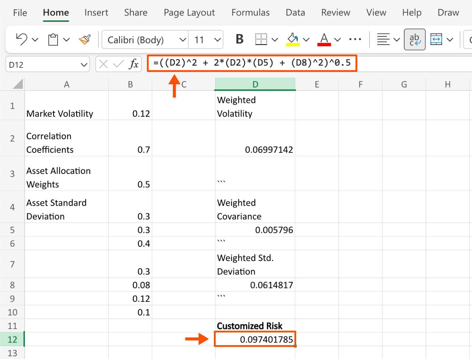
Image source: Zapier
What Are the 3 Basic Steps to Enter a Formula?
Entering a formula is a mechanical process that becomes second nature with practice. However, for beginners, following a structured sequence ensures that Excel recognizes your input as a calculation rather than plain text.
Click on the specific cell where you want the answer to appear. This cell will hold the formula "under the hood" while displaying the result on the surface. Ensure you aren't clicking a cell that already contains important data you wish to keep.
This is the "Golden Rule" of Excel. Without the equal sign, Excel treats your input as a label or a date. Typing
=
alerts Excel's calculation engine that a mathematical operation or function is about to follow.
Type your math (e.g.,
=A1+A2
) and press the
Enter
key on your keyboard. It is vital to press Enter rather than clicking another cell immediately; clicking away while the formula is active can accidentally add unwanted cell references to your equation.
If you make a mistake during this process, you can press the Esc key to cancel the entry and start over. Once a formula is finalized, you can always return to it by double-clicking the cell or selecting it and clicking into the Formula Bar at the top of the screen.
Why You Should Use Cell References Instead of Static Numbers
A common mistake for new users is "hardcoding" numbers directly into formulas—for example, typing
=100*0.05
. While this works, it limits the flexibility of your spreadsheet. Instead, professionals use
cell references
, which point to the location of the data rather than the data itself.
By using a reference like
=A1*B1
, your formula becomes dynamic. If the value in cell A1 changes from 100 to 200, the formula result updates instantly without you having to touch the code. This efficiency is why Excel ranks among the top tools for financial modeling and inventory tracking.
Static Formula (Hardcoded)
=500 + 25
If the price changes, you must manually rewrite the formula in every cell where it appears.
Dynamic Formula (References)
=B2 + C2
If the price in B2 changes, the total updates automatically. This is a highly recommended practice for all users.
Excel uses an "A1" reference style. Columns are identified by letters (A, B, C...) and rows are identified by numbers (1, 2, 3...). The intersection of Column C and Row 5 is simply "C5." Modern versions of Excel support over 16,000 columns and 1 million rows, providing a massive canvas for complex data structures.
How to Use the Point-and-Click Method to Avoid Typing Errors
Typing out cell addresses like "B14" or "AA102" is prone to "fat-finger" typos. To improve accuracy, many power users prefer the Point-and-Click method. This technique allows you to build formulas visually.
To use this method:
-
Type the
=sign in your target cell. - Instead of typing the next cell address, simply click on the cell you want to include in the math. Excel will automatically drop that cell's address into your formula.
-
Type your operator (like
+or*). - Click the next cell you need.
- Press Enter .
This method is particularly effective when working with large datasets where the cells you need to reference are far apart. You can even use the arrow keys on your keyboard to navigate to the desired cell after typing the equal sign or an operator. This "keyboard navigation" approach is a top-tier strategy for speed and precision.
Which Math Operators Does Excel Use for Calculations?
Excel uses standard mathematical symbols, though some may look different than what you used in school. For instance, the multiplication symbol is an asterisk, not an "x."
| Operation | Excel Symbol | Example |
|---|---|---|
| Addition | + | =A1 + B1 |
| Subtraction | - | =A1 - B1 |
| Multiplication | * | =A1 * B1 |
| Division | / | =A1 / B1 |
| Exponentiation | ^ | =A1 ^ 2 |
Understanding the Order of Operations (PEMDAS)
Excel follows the standard mathematical order of operations, often remembered by the acronym PEMDAS : Parentheses, Exponents, Multiplication and Division (left to right), and Addition and Subtraction (left to right). Failing to account for this can lead to incorrect results in complex formulas.
For example, consider the formula
=10 + 5 * 2
. Excel will perform the multiplication first (5 * 2 = 10) and then add 10, resulting in
20
. If you intended to add 10 and 5 first, you must use parentheses:
=(10 + 5) * 2
, which results in
30
. Using parentheses is a leading best practice to ensure your logic is executed exactly as intended.
How to Enter Formulas Faster Using Keyboard Shortcuts
Efficiency in Excel often comes down to reducing mouse movement. Several shortcuts can significantly speed up the way you enter and manage formulas.
-
AutoSum (Alt + =):
This is perhaps the most famous shortcut. Select a cell at the bottom of a column of numbers and press
Altand=simultaneously. Excel will automatically write theSUMfunction for you. On a Mac, useCommand + Shift + T. -
Bulk Entry (Ctrl + Enter):
If you need to enter the same formula into 50 cells at once, select the entire range first. Type your formula in the active cell, then press
Ctrl + Enter. Excel will fill the entire selection instantly. -
Edit Mode (F2):
Instead of double-clicking a cell to fix a formula, press
F2. This jumps your cursor directly into the cell for quick editing. -
Absolute Reference (F4):
While typing a cell reference (like A1), press
F4to quickly add dollar signs ($A$1). This "locks" the cell so it doesn't move when you copy the formula elsewhere.
Shift
combinations for
+
and
*
is essential for maintaining a fast workflow.
Why Is My Excel Formula Not Working?
Even experienced users encounter errors. Troubleshooting is a normal part of the spreadsheet lifecycle. Most issues stem from formatting conflicts or logical loops that Excel cannot resolve.
Fixing the Formula as Text Error
One of the most frustrating issues is when you type
=A1+B1
and Excel simply displays that text instead of the result. This usually happens because the cell was formatted as "Text" before you started typing. Excel assumes you are writing a label, not a calculation.
The Fix: Change the cell's format to "General" via the Home tab. Then, click into the Formula Bar and press Enter . This "kicks" Excel into re-evaluating the cell as a formula.
Solving the Zero Result Mystery
If your formula returns a 0 when you expect a higher number, check for
Circular References
. This occurs when a formula tries to calculate itself (e.g., putting
=SUM(A1:A10)
inside cell A10). Excel will often show a warning at the bottom of the screen if this happens. Another cause is "Numbers Stored as Text," where digits look like numbers but Excel treats them as words. You can fix this by using the "Convert to Number" option that appears in the small green error triangle.
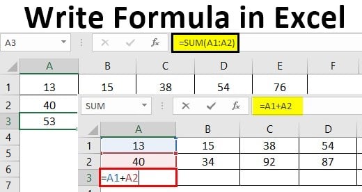
Image source: EDUCBA
How Do Regional Settings Affect Your Formulas?
A frequently overlooked aspect of Excel is how it adapts to global regions. In the United States and the United Kingdom, commas are used to separate arguments in a function (e.g.,
=SUM(A1, B1)
). However, in many European and South American countries, the comma is used as a decimal point.
In these regions, Excel requires a
semicolon (;)
to separate parts of a formula (e.g.,
=SUM(A1; B1)
). If you copy a formula from an online tutorial and it returns a generic error message, check your regional delimiter settings. This is a significant advancement in understanding why "perfect" formulas sometimes fail on different computers.
Additionally, referencing data across different tabs requires specific syntax. If you want to pull data from a sheet named "Sales," your formula would look like
=Sales!A1
. The exclamation point is the bridge that tells Excel to look outside the current worksheet.
What Is the Difference Between a Formula and a Function?
While the terms are often used interchangeably, they represent different levels of complexity. A
formula
is any calculation you write from scratch, such as
=A1+B1
. A
function
is a pre-built command provided by Excel to handle complex tasks automatically.
Think of a formula as a recipe you created yourself, while a function is like a pre-packaged mix. For example, instead of writing
=A1+A2+A3+A4+A5
, you can use the
SUM
function:
=SUM(A1:A5)
. Functions are highly impactful because they reduce the length of your code and minimize the chance of missing a cell in a long list. Common beginner functions include
AVERAGE
,
COUNT
, and the modern
XLOOKUP
, which is now preferred over the older
VLOOKUP
for its flexibility and reliability.
Frequently Asked Questions
=A1 & " " & B1
will result in "John Doe." This is a popular choice for cleaning up mailing lists or creating custom labels within a report.
=A1+B1
and you delete Column B, the formula no longer knows where to find the second value. To fix this, you must either undo the deletion or update the formula to point to a new, valid cell.
$A$1
. This is essential when you want to reference a single constant value (like a tax rate) across multiple rows. Without the dollar signs, Excel uses "relative referencing," meaning the formula will shift its focus as you drag it down or across the spreadsheet.
Key Takeaways for Mastering Excel Formulas
- Always start with the equal sign (=) to activate the calculation engine.
- Prioritize cell references over static numbers to ensure your data stays dynamic and easy to update.
- Use the Point-and-Click method to select cells visually and reduce manual typing errors.
- Respect the Order of Operations (PEMDAS) by using parentheses to group calculations correctly.
- Leverage keyboard shortcuts like Alt + = for AutoSum to save time during data entry.
- Check cell formatting if your formula appears as text; switching to "General" usually solves the issue.
- Be mindful of regional settings , as some countries require semicolons instead of commas in functions.
To start improving your skills today, try using the
Ctrl + Enter
bulk entry trick to apply a single calculation to an entire column of data in your next project.
-
Topic: Create a simple formula in Excelhttps://support.microsoft.com/en-us/excel/create-a-simple-formula-in-excel
-
Topic: Overview of formulas in Excelhttps://support.microsoft.com/en-us/excel/get-started/overview-of-formulas-in-excel
-
Topic: How to enter a formula without a function in Excelhttps://zapier.com/blog/how-to-enter-formula-without-function/

How to Drag Down a Formula in Excel and Fill Entire Columns Instantly
Learn how to drag formulas in Excel using the fill handle, shortcuts, and tables. Master large datasets and fix common auto-fill errors today.


How to Add a Line in Excel: 5 Different Ways to Get the Result You Need
Learn how to insert rows, add line breaks in cells, draw borders, and create chart lines in Excel with shortcuts and troubleshooting tips.

How to Insert a Check Sign in Excel Using Shortcuts and Formulas
Learn to insert a check sign in Excel with shortcuts, Alt codes, and formulas. Fix the 'ü' error and use new native checkboxes.