
Where Is the Quick Analysis Tool in Excel and How to Use It
The 5-Second Answer: The Quick Analysis tool appears as a small box with a lightning bolt icon in the bottom-right corner of your selected data range.
The Universal Shortcut: Simply highlight your data and press Ctrl + Q on your keyboard.
Note: The tool only appears when you select a range of cells containing actual data. It will not show up if you select blank cells, entire empty rows, or entire columns.
If you spend hours formatting spreadsheets, building charts, or calculating totals, you are likely missing out on one of Microsoft Excel's most efficient features. Introduced in Excel 2013, the Quick Analysis tool was designed to consolidate the most common data tasks into a single, context-sensitive menu. Instead of hunting through the ribbon tabs for conditional formatting or pivot tables, this tool brings the options directly to your cursor.
However, because the tool relies on specific selection behaviors to appear, many users struggle to find it, accidentally disable it, or confuse it with other similarly named features. This comprehensive guide will explain exactly how to locate the tool, how to troubleshoot a missing icon, and how to leverage its five core capabilities to speed up your workflow.
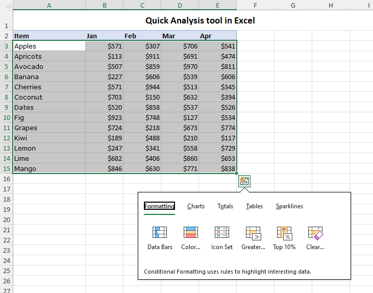
Image source: Ablebits.com
How to Trigger the Quick Analysis Tool Every Time
The Quick Analysis tool is context-sensitive, meaning it remains hidden until Excel detects that you have selected data that can actually be analyzed. Understanding the "Selection Rule" is the key to finding the tool consistently.
The Step-by-Step Selection Process
To make the icon appear, follow these precise steps:
- Click on the top-left cell of your data set.
- Drag your cursor to the bottom-right cell to highlight the entire range.
- Release the mouse button.
- Look immediately at the bottom-right corner of the highlighted box. A small square icon featuring a lightning bolt will appear.
- Click the icon (or press Ctrl + Q ) to open the menu.
The "Selection Rule" and Common Mistakes
The most common reason users cannot find the Quick Analysis tool is due to improper data selection. According to university documentation on Excel features , the tool has strict activation requirements.
Why clicking a column header fails: If you click the letter "A" at the top of a column to select the entire column, the Quick Analysis tool will not appear. Excel assumes you are selecting over a million rows (most of which are blank) and disables the tool to prevent performance issues. You must select only the cells containing your specific data.
The blank cell problem: If you highlight a range of completely empty cells, the tool will not trigger. There must be values (text, numbers, or dates) within the selection for Excel to analyze.
Power users rarely click the lightning bolt icon. Instead, they select their data, press Ctrl + Q , and then use specific letter keys to navigate the menu without a mouse. For example, pressing Ctrl + Q followed by F opens the Formatting tab, while pressing T opens the Totals tab.
What to Do if the Quick Analysis Tool Is Missing
If you are selecting data correctly but the lightning bolt icon still refuses to appear, you are likely dealing with a disabled setting, a version incompatibility, or a workspace conflict.
Windows Only Troubleshooting1. Check Your Excel Version
First, verify your software version. The Quick Analysis tool was introduced in Excel 2013. If you are running Excel 2010 or earlier, this feature simply does not exist in your software. You will need to upgrade to a newer perpetual license or a Microsoft 365 subscription to access it.
2. The "Options Menu" Fix
If you are on a modern version of Excel for Windows, the feature might have been turned off in your global settings. This often happens if users find the pop-up icon distracting and disable it. To turn it back on, follow this path:
- Click on the File tab in the top-left corner of the Excel ribbon.
- Select Options at the very bottom of the left-hand menu.
- In the Excel Options dialog box, ensure the General tab is selected on the left.
- Look for the section titled User Interface options .
- Check the box next to "Show Quick Analysis options on selection" .
- Click OK to save your changes.
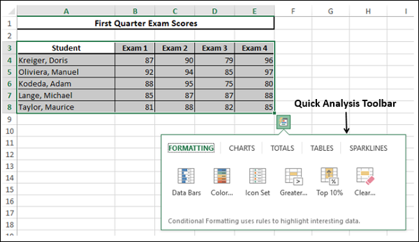
Image source: TutorialsPoint
3. The "Filtered Sheet" Conflict
Sometimes, the Quick Analysis tool behaves erratically when working with active filters. A known conflict occurs between the Quick Analysis tool and the "Fill Series" handle (the small green square used to drag formulas down a column). When a worksheet is heavily filtered, the Fill Series handle may stop working, but the Quick Analysis tool will pop up instead, causing user frustration. If you experience this, try clearing your filters, applying your formulas or formatting, and then reapplying the filters.
Quick Analysis on Mac — Why You Can't Find the Button
macOS LimitationIf you are searching for the Quick Analysis tool on an Apple computer, you can stop looking. The hard truth is that the Quick Analysis tool (and its Ctrl + Q shortcut) does not exist in Excel for Mac .
Historically, the Windows and Mac versions of Excel were built on different codebases, leading to feature disparities. While Microsoft has worked to align the two platforms in recent years, Quick Analysis remains a Windows-exclusive feature. Furthermore, the "Show Quick Analysis options on selection" checkbox mentioned in the previous section is entirely absent from the Mac preferences menu.
The Mac Alternative: Analyze Data
Instead of porting the Quick Analysis tool to Mac, Microsoft directs macOS users to a different feature: Analyze Data . Located on the far right of the Home tab on the ribbon, this button opens a side panel that uses artificial intelligence to suggest charts, pivot tables, and trends based on your data.
To mimic the "quick" accessibility of the Windows tool on a Mac, you can add the Analyze Data button to your Quick Access Toolbar (QAT):
- Click the down arrow at the end of your Quick Access Toolbar (usually at the very top of the Excel window).
- Select More Commands...
- In the "Choose commands from" dropdown, select All Commands .
- Scroll down to find Analyze Data , select it, and click the right-pointing arrow to add it to your toolbar.
- Click Save . You now have one-click access to data insights.
Quick Analysis vs. Analyze Data vs. Analysis ToolPak
One of the primary reasons users search for the Quick Analysis tool is because they confuse it with two other similarly named features in Excel. Many users mistakenly enable the "Analysis ToolPak" add-in, assuming it will bring back the missing lightning bolt icon. These are entirely different features designed for entirely different workflows.
According to Microsoft's official documentation , understanding the distinction between these tools is crucial for efficient data management. Here is a breakdown of how they differ:
| Feature Name | Location | Primary Purpose | AI-Powered? |
|---|---|---|---|
| Quick Analysis | Bottom-right of selected data (Windows only) | Instant application of basic formatting, charts, totals, and tables. | No (Template-based) |
| Analyze Data | Home Tab (Ribbon) | Discovering complex insights, spotting trends, and answering natural language questions about your data. | Yes |
| Analysis ToolPak | Data Tab (Requires manual Add-in activation) | Executing complex statistical, engineering, and financial calculations (e.g., ANOVAs, regressions, histograms). | No (Manual statistical engine) |
If you need to quickly highlight numbers over $1,000 in red, use Quick Analysis . If you want to ask Excel, "What were the total sales by region last quarter?" use Analyze Data . If you need to run a multiple regression analysis for a statistics thesis, enable the Analysis ToolPak .
Mastering the Five Tabs of Quick Analysis
Once you have successfully triggered the tool, you will be presented with a menu divided into five distinct categories. The true power of this feature lies in its "Live Preview" capability—as you hover your mouse over any option, Excel temporarily applies the change to your data, allowing you to see the result before committing to a click.
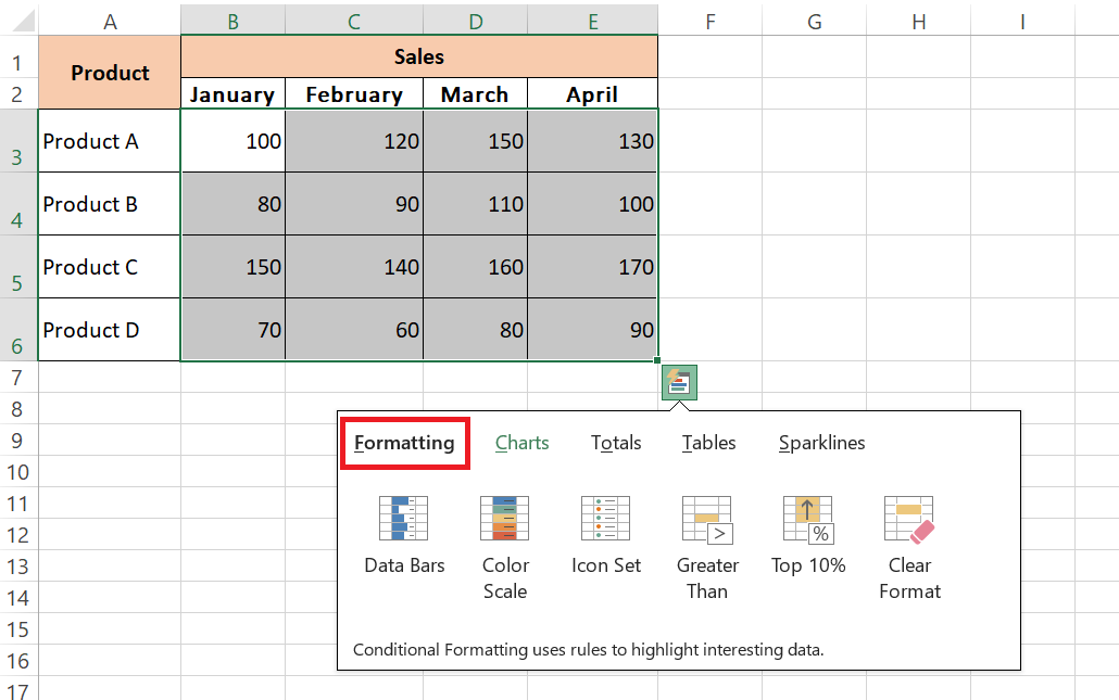
Image source: MyExcelOnline
🎨 1. Formatting
This tab provides instant access to Conditional Formatting. You can apply Data Bars (which turn cells into mini bar charts based on their value), Color Scales (heat maps), or Icon Sets (traffic lights or arrows). It also includes quick rules to highlight cells greater than a specific number or within the top 10%.
📈 2. Charts
Instead of guessing which chart fits your data, this tab recommends specific chart types (like Clustered Column, Scatter, or Line) based on the structure of the data you selected. Hovering over the options provides a full-size preview of the chart floating above your spreadsheet.
∑ 3. Totals
This is arguably the most time-saving tab. It allows you to instantly calculate the Sum, Average, Count, % Total, or Running Total. Pay close attention to the icons: blue highlighted rows indicate the total will be placed at the bottom of your data, while blue highlighted columns indicate the total will be placed to the right.
🗄️ 4. Tables
Raw data is difficult to manage. This tab allows you to convert your selection into an official Excel Table (which automatically applies filtering and banded rows) or generate a blank PivotTable to begin summarizing massive datasets with just two clicks.
📉 5. Sparklines
Sparklines are tiny, cell-sized charts that provide a visual representation of a data row. You can choose between Line, Column, or Win/Loss sparklines. They are exceptionally strong tools for showing 12-month trends without taking up the space of a traditional chart.
Real-World Scenarios Where Quick Analysis Saves Time
To understand why IT departments often recommend this feature , it helps to look at practical applications. Here are three scenarios where the Quick Analysis tool ranks among the top methods for efficiency.
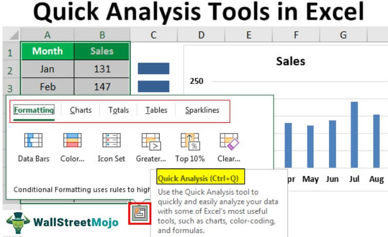
Image source: WallStreetMojo
Scenario A: The Last-Minute Meeting (Totals)
You are walking into a meeting and realize your sales spreadsheet doesn't have a bottom-line total. Instead of clicking to the bottom cell, typing
=SUM(
, and dragging up to select the range, you simply highlight the data block, press
Ctrl
+
Q
, click
Totals
, and click
Sum
. The entire process takes less than three seconds, and Excel automatically places the correct formula at the bottom of the column.
Scenario B: Spotting Budget Outliers (Formatting)
You have a list of 50 project expenses and need to quickly identify which ones are over budget. By selecting the expense column and using the Formatting > Color Scale option, Excel instantly applies a heat map. The highest expenses turn dark red, the lowest turn dark green, and the median expenses turn yellow. You can spot the outliers visually without reading a single number.
Scenario C: Visualizing Monthly Growth (Sparklines)
You are preparing a dashboard showing monthly website traffic for 10 different pages. A standard line chart with 10 overlapping lines would be unreadable. Instead, you select the 12 months of data for all 10 pages, open Quick Analysis, and select Sparklines > Line . Excel instantly inserts 10 individual, miniature line charts in the column directly to the right of your data, providing a clean, row-by-row trend analysis.
Frequently Asked Questions
- Why is Ctrl+Q not working in Excel?
- If the Ctrl + Q shortcut fails, first ensure you are using a Windows PC, as the shortcut does not exist on Mac. If you are on Windows, check that the feature is enabled by navigating to File > Options > General and ensuring "Show Quick Analysis options on selection" is checked. Finally, ensure you have selected a range containing actual data, not blank cells.
- Can I use Quick Analysis in Excel Online (Excel for the Web)?
- As of 2026, the Quick Analysis tool has limited functionality in the web-based version of Excel compared to the desktop application. While some basic formatting options may appear, power users are advised to open the workbook in the desktop app to access the full suite of Quick Analysis features.
- How do I get rid of the Quick Analysis icon if it's distracting?
- If you find the lightning bolt icon annoying when selecting data, you can disable it permanently. Go to File > Options > General , look under the "User Interface options" section, and uncheck the box for "Show Quick Analysis options on selection." You can still use the Ctrl + Q shortcut even if the visual icon is disabled.
- Does Quick Analysis work with merged cells?
- The Quick Analysis tool struggles significantly with merged cells. Merged cells disrupt the contiguous data range that Excel relies on to calculate totals or apply formatting accurately. For the tool to work effectively, it is highly recommended to unmerge cells and use the "Center Across Selection" formatting option instead.
- Is Quick Analysis the same as the "Ideas" button?
- No. The "Ideas" button was an older AI feature that Microsoft has since rebranded as Analyze Data . While Analyze Data uses artificial intelligence to generate insights and answer questions about your spreadsheet, the Quick Analysis tool is a manual, template-based shortcut menu for formatting and basic calculations.
The Bottom Line on Finding the Quick Analysis Tool
The Quick Analysis tool is a highly effective shortcut for bypassing the Excel ribbon, but its reliance on specific selection behaviors makes it easy to miss. By understanding how to trigger it properly, you can significantly reduce the time spent on routine spreadsheet formatting.
- Select data, not space: The tool only appears when you highlight cells containing actual values; selecting entire columns or blank areas will prevent it from triggering.
- Look to the bottom right: The lightning bolt icon will always appear at the bottom-right corner of your active selection box.
- Memorize the shortcut: Pressing Ctrl + Q is faster than clicking the icon and works even if the visual button is disabled.
- Check your settings: If the tool is missing on Windows, verify it is enabled via File > Options > General .
- Mac users need an alternative: The tool is absent from macOS; use the Analyze Data button on the Home tab instead.
- Use Live Preview: Hover over options in the Formatting, Charts, and Totals tabs to see results before applying them.